Here is a link to the C-source of the program.
The following links are to archives which have to be unpacked with
`tar':
This contains just the sources, makefile
and documentation.
Sources and a
compiled version for DEC alpha.
Sources and a
compiled version for DEC Ultrix.
Sources and a
compiled version for SUN Solaris.
Sources and a
compiled version for Free BSD on a PC.
Sources and a
compiled version for Linux on a PC.
Be careful with the Linux version because it is known to occasionally
produce wrong results, but we are not sure whether this is the fault
of Linux or of the Pentium (`Intel inside') !
This program may be freely distributed and changed,
provided that your changes are marked clearly and
the notice in the header of the source remains unchanged.
The algortithm used in this program is described mainly
in appendix C of [1].
Equation numbers here and in the source refer to this paper.
There are the following differences in notation between this program
and our paper [1]:
- The program starts to number the sites with 0 while in
our paper we start to count with 1. Thus, in the program
x runs from 0 to N-1 in contrast to the range [1,N].
This has also the
effect that the notion of even and odd are reversed in the
program with respect to the paper.
- The program uses the notation <n_x> for the expectation
value of the particle density while in the paper we used
the notation <\tau_x>.
The program is called from the command line, usually by typing
`matprod'. A file which is used to store the results has to
be given as an argument on the command line. Several options
(which all start with a `-') may be added.
The specification of this output file on the command line is compulsory.
Options in the command line may but need not be specified.
We are now going to discuss the possible options a bit.
The options for setting the parameters are:
- -a#
- Set the input probability \alpha equal to #.
- -b#
- Set the output probability \beta equal to #.
- -g#
- Set the output probability \gamma equal to #.
- -d#
- Set the input probability \delta equal to #.
- -p#
- Set the probability p for hopping to the right equal to #.
- -q#
- Set the probability q for hopping to the left equal to #.
Above, `#' refers to a floating point number between 0 and 1.
Either all numbers in the set {p,\alpha,\beta} or all in
the set {q,\gamma,\delta} must be strictly positive (and preferrably not
too small).
- -N#
- Set the chain length N equal to #. Here # is supposed to be a positive
even integer. How large N can be
chosen depends on the floating point accuracy as well as on
the available memory and CPU time. Usually, N=100 causes no problems.
A computation of a two-point function takes of the order N times
longer than the computation of a profile. So, although
profiles can still be computed for N > 300, it is not
very sensible to go beyond N=200 for the two-point functions.
Going beyond N=400 will usually not be possible due to lack
of main memory.
If too many probabilities are too small, it is possible that
the numerical range for floating point arithmetics is exceeded
already before these limits are reached.
If these parameters are not specified on the
command line, they are entered interactively after starting
the program. The program checks that the parameters are in
a valid range and, if necessary, rejects the input.
The following options are used to control the correlation functions
computed:
- -c
- Compute the connected two-point function <n_x n_y> - <n_x><n_y>.
- -f
- Compute the full two-point function <n_x n_y>. This is the default.
- -j
- Compute just the density-profile <n_x> and no two-point functions.
If this option is specified, `-c' and `-f' have no effect.
- -t
- Compute two-point functions. Then the profile is given by the diagonal,
i.e. <n_x> = <n_x n_x>. This is the default.
These options are used to decide whether to perform cmputations only
on the even or the odd sublattice or on both:
- -e
- Compute quantities only on the even sublattice, i.e. only n_x. This is the default.
- -o
- Compute quantities only on the odd sublattice, i.e. only \hat{n}_x.
- -y
- Compute quantities everywhere on the lattice, i.e. both n_x and \hat{n}_x.
Here are finally a few options which control some details:
- -m
- Reverse the sign of connected two-point function. This has an effect
only if used together with the option `-c'. The purpose of this option
is that one may wish to plot the connected two-point function on
a logarithmic scale, but <n_x n_y> - <n_x><n_y> can be
negative.
- -r
- Use a spatially reversed system for internal computations.
- -s
- Use standard order in space for internal computations.
If `-r' or `-s' is not specified, the decision is taken automatically. These
two options are important because they control how large the numbers
get in the internal computations, but have no effect on the input or
output. If the program terminates with a floating exception after
computing at least some s(x), try to use the other option (or if the
decision was taken automatically, try these two options). If in either
case a floating exceptions is produced while doing the algebra, it is
not possible to work with the chosen parameters with this program.
Then either use a shorter chain length or try to modify the probabilities
slightly.
After the program is started it prints all parameters. Then it computes
the associated \hat{\kappa}-functions and determines which phase they
correspond to. The analytic results of [1] for the
quantities in the thermodynamic limit are also evaluated
and displayed. If a spatially reversed system is used internally,
the program now informs the user. Next, the s_x are computed for x <= N and printed.
Then, the results for the current J = <W| C^(n-1) |V> / <W| C^n |V>
are computed and printed for system sizes n <= N. Finally, the main computations
(profile and possibly the two-correlation function) are performed and
stored in the file specified on the command line. Most of the information
displayed directly after the start of the program is also included
as a comment at the top of this output file.
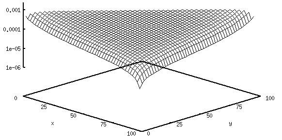
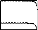
We wish to generate the figure presented at the top of this WWW page.
First, the data file must be generated using the program discussed here.
Assume that you have an executable version which is called `matprod'.
Then this is the correct command which includes all parameters on the
command line:
matprod -n100 -p0.75 -q0.25 -a0.5 -b0.6 -g0.1 -d0.2 tpfc.plt -c -m
The option `-c' switches to the generation of the connected two-point
function. The option `-m' has been added because we wish to plot
on a logarithmic scale, but the values turn out to be negative.
The resulting file `tpfc.plt' is now plotted using gnuplot's
`splot' command. Here are
the basic commands to be performed by gnuplot (no fancy labeling of
axes etc.):
  set xrange [0:100]
  set yrange [0:100]
  set zrange [0.000001:0.001]
  set log z

  set parametric
  set view ,45

  splot "tpfc.plt" w l
Now you should see something which looks more or less the same as the
above figure.
Now we present figures of a few densities profiles obtained with
this program (mostly for N=100) and discuss their physical implications.
These density profiles can also be obtained by Monte-Carlo simulations
[2], but (at least for system sizes of a few hundred
sites) the computation using the algebra is not only more
accurate but also much faster.
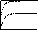
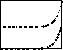
An illustration of finite-size effects
in the maximal current phase.
Shown is the density on the even sublattice for N=100, N=200, N=300 and
N=400.
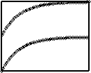
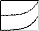
Some density profiles in the high density phase.
All of them are for
\hat{\kappa}_{+}(\alpha, \gamma) \hat{\kappa}_{+}(\beta, \delta) > 1.
The lines are based on
the following results of [1]: Eq. (4.2a) for the
densitites <n_x> and <\hat{n}_x> and eq. (4.6) for exp(1/\zeta)
encoding the correlation length \zeta. Just the amplitudes of
the boundary effects have been fitted. This demonstrates the
general validity of these results also off the one- and two-dimensional
representations.
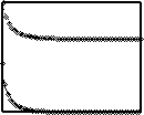
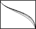
A density profile in the high density phase with
\hat{\kappa}_{+}(\alpha, \gamma) \hat{\kappa}_{+}(\beta, \delta) < 1.
Eq. (4.2a) still applies but eq. (4.6) for the correlation length \zeta
is not valid any more.
Summarizing the results of the previous four figures we conclude that
one should probably make a subdivision of phase I in Fig. 3 of [1]
into two subphases which are separated by the one-dimensional line.
This generalizes the subdivision observed in [3] for special values of the
rates in the sequential limit. For more details see also [2].
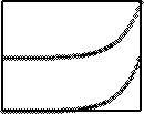
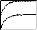
Some density profiles in the low density phase.
All of them are for
\hat{\kappa}_{+}(\alpha, \gamma) \hat{\kappa}_{+}(\beta, \delta) > 1.
The lines encode the following results of [1]: Eq. (4.2b) for the
densitites <n_x> and <\hat{n}_x> and eq. (4.6) for exp(1/\zeta)
corresponding to the correlation length \zeta. Just the amplitudes of
the boundary effects have been fitted. This demonstrates the
general validity of these results also off the one- and two-dimensional
representations.
A density profile in the low density phase with
\hat{\kappa}_{+}(\alpha, \gamma) \hat{\kappa}_{+}(\beta, \delta) < 1.
Eq. (4.2b) still applies but eq. (4.6) for the correlation length \zeta
is not valid any more.
Summarizing the results of the previous four figures we conclude that
like in te case of the high denisty phase (phase I)
one should probably make a subdivision of phase II in Fig. 3 of [1]
into two subphases which are separated by the one-dimensional line.
This generalizes the subdivision observed in [3] for special values of the
rates in the sequential limit (see also [2]).
- A. Honecker, I. Peschel, Matrix-Product States for a
One-Dimensional Lattice Gas with Parallel Dynamics,
J. Stat. Phys. 88 (1997) 319
(slightly shortened and restructured version of
preprint cond-mat/9606053)
- N. Rajewsky, L. Santen, A. Schadschneider, M. Schreckenberg,
The Asymmetric Exclusion Process: Comparison of Update
Procedures, J. Stat. Phys. 92 (1998) 151
(preprint
cond-mat/9710316)
- B. Derrida, M.R. Evans, V. Hakim, V. Pasquier, Exact
Solution of a 1D Asymmetric Exclusion Model Using a Matrix
Formulation, J. Phys. A: Math. Gen. 26 (1993)
1493-1518
June, 12th, 1996 - last modified on December, 13th, 1999
a.honecker@tu-bs.de